Pixel-based supervised image classification
Author: Jan Haas - Last update: 2023-09-20
Citation:
Haas, J. (2024). Pixel-based supervised image classification. Zenodo. doi.org/10.5281/zenodo.10687552
Introduction
This tutorial aims at familiarizing the user with image processing and image classification to obtain land use/land cover (LULC) data that can be used to describe landscapes from an archaeological perspective. The user is introduced to image processing using Principal Component Analysis (PCA) in order to reduce data dimensionality and to pixel-based texture analysis using Gray Level Co-occurrence Matrix (GLCM), followed by pixel-based supervised image classification in ESA SNAP. Furthermore, the user will learn how to perform image reclassification in QGIS and to evaluate the reliability of the classification result through accuracy assessment in form of a confusion/error matrix using a script in RStudio. After completing this tutorial, the user should be able to derive LULC information from satellite data and evaluate the accuracy and reliability of the classification. The tutorial is based on straight-forward user-friendly solutions using free and open-source programs.
Tutorial
In order to complete the tutorial, the user will have to install three programs. Apart from ESA SNAP, the tutorial makes use or RStudio and QGIS. Go to the websites and choose the appropriate installers for your system. For the installation of SNAP, it is referred to the tutorial Satellite image processing. Following this tutorial, the user will learn how to perform image processing and pixel-based classification in ESA SNAP, export data for reclassification in QGIS and perform accuracy assessment in RStudio.
1. Image processing in SNAP
1.1 Open SNAP and add data
Start SNAP and got to File > Open Product and browse to a previously created file, e.g., subset_0_of_S1-S2_stack.dim from the previous tutorial Satellite image processing.
1.2 Perform Principal Component Analysis (PCA)
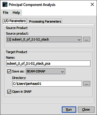
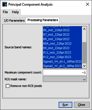
Go to the Raster tab and click on Image Analysis and choose Principal Component Analysis. Choose the satellite image as source file and save the output in the same directory. Keep the automatically generated file name ….stack_pca (Figure 1). Save in the BEAM-DIMAP format. Go to the processing parameters, choose all the band names but leave the other fields untouched (Figure 2). Click on Run to generate the file.
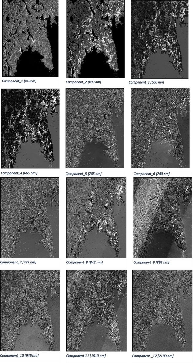
The output of the PCA is displayed in the following figure (Figure 3). Note that the discrimination between land cover in the first bands 1-4 is most prominent. The redundancy of data increases gradually from band 1 to 12 and visual inspection suggests that only using band 1-4 for classification is sufficient.
1.3 Texture analysis with Gray Level Co-occurrence Matrix (GLCM)
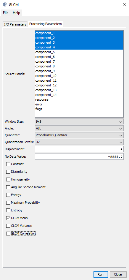
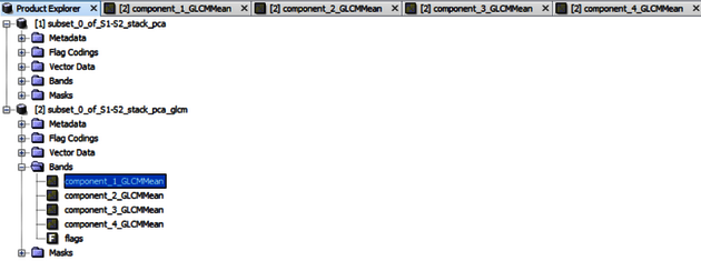
Go to the Raster tab and click on Image Analysis > Texture Analysis and choose Gray Level Co-occurrence Matrix (GLCM). Choose bands 1-4 as the processing parameters and GLCM Mean (Figure 4). Keep all other parameters set to default. Choose the latest image as source file after PCA, i.e., stack_pca and save the file in the same directory. Keep the automatically generated file name … _stack_pca_glcm. Save in the BEAM-DIMAP format. Click on Run to generate the file.
The output of the GLCM operation is displayed in Figures 5 and 6.

2. Image classification in SNAP
2.1 Create a False Colour Composite (FCC)
Go to the Window tab and click on Open RGB Image Window. Click on […] to Red and choose the original image, e.g., subset_0_of_S1-S2_stack.dim as product and choose Band 8 (Figure 7). Then do the same for Green (choose band 4) and Blue (choose the band 3) (Figure 8). Click on OK to generate the RGB Image (Figure 9).
2.2 Synchronizing image views
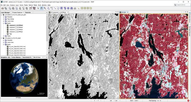
Go to the Window tab and click on Tile Horizontally, have only two labels open, the RGB image (FCC visualization) and a component of the GLCM operation. Then go to View tab and click on Synchronize Image Cursors and Views. The output of this processing is displayed in Figure 10.
2.3 Training data collection
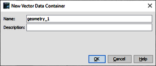
Go to the Vector tab and click on New Vector Data Container (Figure 11). Start to create samples. Choose an appropriate shape for collecting samples from the tool bar. Highest flexibility is granted with the Polygon drawing tool (highlighted in Figure 12).

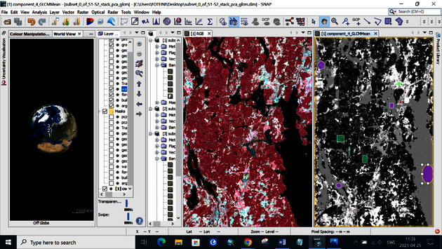
Several samples need to be taken for every vector. Start by generating 10 different samples per vector well distributed over the image, capturing as many variations in a land cover class as possible, e.g., water should contain sea, lake, river, turbid, shallow and so forth. If the classes are very different from each other in the spectral response, it is best to create several vectors for the same class, i.e., agriculture (vegetated field) and agriculture (bare field). Figure 13 displays training samples for the classes water, built-up, forest and agriculture/open land.
2.4 Supervised classification
Go to the Raster tab and click on Classification > Supervised Classification and choose Random Forest Classifier. Click on

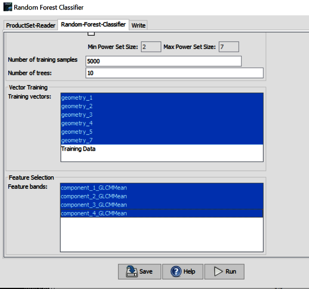
and load the …_stack_pca_glcm image to the ProductSet-Reader. Then choose the training vectors and the feature bands that have been used (Figure 14). Click on Run to generate the file. Go to the Product Explorer Label, choose the ….__pca_glcm_RF, click on Band and then Labelled classes in order to display the classification result (Figure 15).
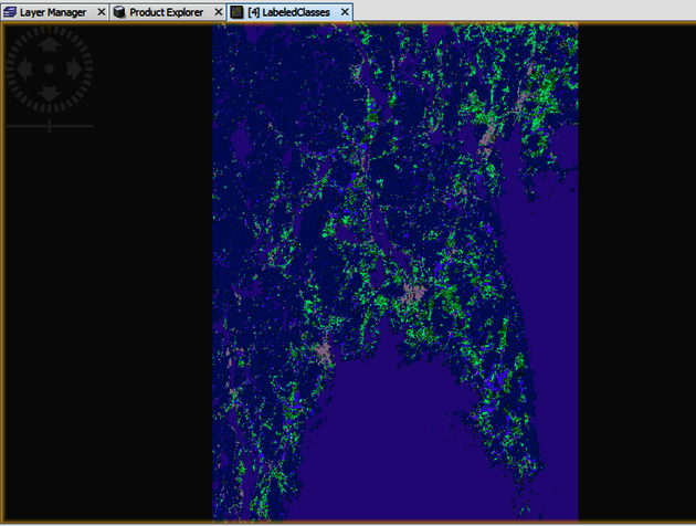
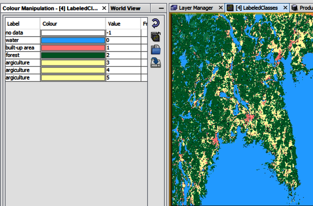
Click on Labeled Classes to open the Colour Manipulation window (Figure 16). In this window you can change name and colour of the labels. Figure 17 displays the output after the changes.

Go to the File tab and click on Export and choose GeoTIFF and give it an appropriate name, e.g., classified_subset.tif.
3. Accuracy Assessment
For accuracy assessment we are interested in comparing the LabledClasses band to the reference data. We will thus only investigate one band in QGIS.
3.1 Creating a one band subset
Open QGIS and drag and drop the classified image classified_subset.tif into the main frame. Right click on the classified_subset.tif layer and choose Properties (Figure 18). Change Render type to Singleband gray and choose Band 2 in the Gray Band field (Figure 19). Click OK.
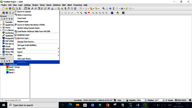
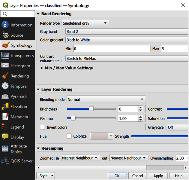
Go to the Raster tab and click on Conversion and choose Translate. In the Translate window, perform the following tasks (Figure 20):
1. Select your input layer.
2. Expand Advanced Parameters.
3. Select the output path and write an output file name, e.g., classified_subset_temp.
Write [-b 2] to the Additional command-line parameter.
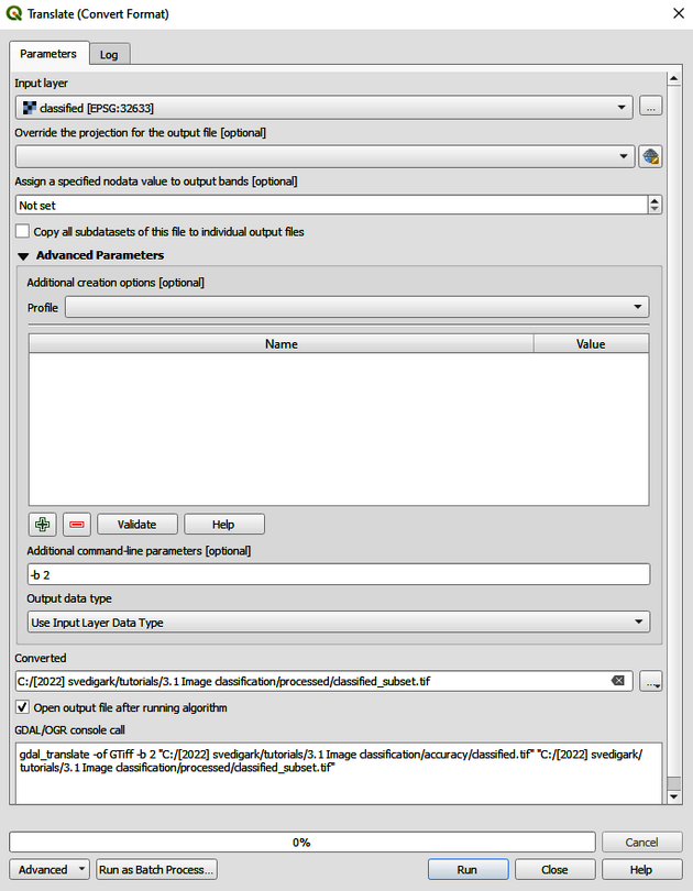
3.2 Reclassification in QGIS
In order to compare the classified data to the reference data, we need to make sure that all classes have the same raster values. We need to reclassify our data according to the reference data into the following classes: 1 Water; 2 Built-up; 3 Forest; 4 Agriculture/open land. Write on the Type to locate tab in the at the bottom of the frame Reclassify by Table. Change the parameters as they are displayed on Figure 21 and save it as reclassified_subset. Make sure that you use min <= value <= max as Range boundaries.
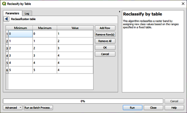
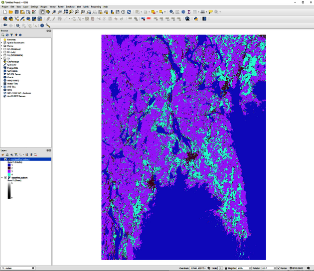
Right click on classified_subset_temp, click on Export and choose Save As. Export raster to .geotiff and name it reclassified_subset.
3.3 Create a confusion/error matrix in RStudio
Open RStudio (Figure 23) and click on the little green plus in the upper left corner and choose RScript.
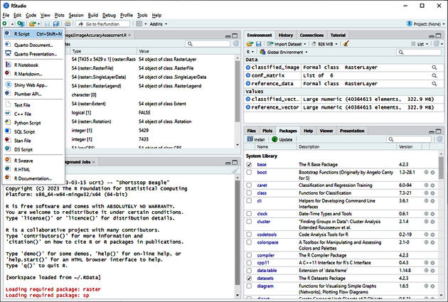
Copy and paste the following code into Rstudio. The code was generated through ChatGPT 4.0 and modified for the tutorial. If you need a particular modification or want to use other means of accuracy assessment, consult ChatGPT for adaptation. The reference data reference_reclassified.tif is provided alongside this tutorial.
Code for creating a confusion matrix in R:
# Install and load required packages
if (!requireNamespace("caret", quietly = TRUE)) {
install.packages("caret")
}
if (!requireNamespace("raster", quietly = TRUE)) {
install.packages("raster")
}
library(caret)
library(raster)
# Load classified image (replace "path/to/classified_image.tif" with the actual file path)
classified_image <- raster("C:/temp/reclassified_subset.tif")
# Load reference data (replace "path/to/reference_data.tif" with the actual file path)
reference_data <- raster("C:/temp/reference_reclassified.tif")
# Check if dimensions and extent of the rasters match
if (compareRaster(reference_data, classified_image)) {
# Convert rasters to vectors
classified_vector <- as.vector(classified_image[])
reference_vector <- as.vector(reference_data[])
# Create confusion matrix
conf_matrix <- confusionMatrix(as.factor(classified_vector), as.factor(reference_vector))
# Print confusion matrix
print(conf_matrix)
} else {
cat("The dimensions or extents of the rasters do not match.")
}
Adjust the path where reference and classified images are located and run the code. Figure 24 shows the results of accuracy assessment.
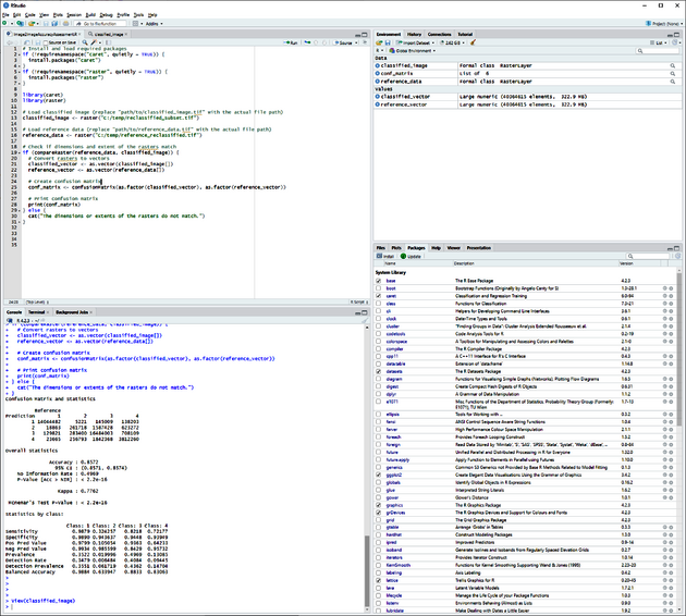
The results should look like this:
Confusion Matrix and Statistics
Reference
Prediction 1 2 3 4
1 14044482 5221 145009 138203
2 18863 261718 1587428 623272
3 129821 283400 16484003 708109
4 23665 256793 1842368 3812260
Overall Statistics
Accuracy : 0.8572
95% CI : (0.8571, 0.8574)
No Information Rate : 0.4969
P-Value [Acc > NIR] : < 2.2e-16
Kappa : 0.7762
Mcnemar's Test P-Value : < 2.2e-16
Statistics by Class:
Class: 1 Class: 2 Class: 3 Class: 4
Sensitivity 0.9879 0.324257 0.8218 0.72177
Specificity 0.9890 0.943637 0.9448 0.93949
Pos Pred Value 0.9799 0.105054 0.9363 0.64233
Neg Pred Value 0.9934 0.985599 0.8429 0.95732
Prevalence 0.3522 0.019996 0.4969 0.13085
Detection Rate 0.3479 0.006484 0.4084 0.09445
Detection Prevalence 0.3551 0.061719 0.4362 0.14704
Balanced Accuracy 0.9884 0.633947 0.8833 0.83063
When communicating the results from the classification, present the figures that are marked in red, i.e., the actual confusion matrix, overall accuracy and Kappa value. From the confusion matrix, calculate and report even user’s accuracy and producer’s accuracy as measures on commission and omission errors according to this guide.
How to
This section covers some topics that need consideration from the analyst when performing image analysis, image classification and accuracy assessment.
Image Processing
Principal Component Analysis (PCA)
PCA is a widely used technique for dimensionality reduction and feature extraction in data analysis. It aims to find a set of orthogonal axes, called principal components, that capture the maximum variance in the data. These components can be used to project the original data points into a lower-dimensional space, reducing noise and redundancy. The following steps are part of a PCA:
• Prepare the dataset: Organize the data as an n x m matrix, where n is the number of samples (data points) and m is the number of features (dimensions). Ensure that the data is normalized or standardized, meaning each feature should have a mean of zero and, ideally, unit variance.
• Calculate the covariance matrix: Compute the covariance matrix (C) of the data. This is an m x m symmetric matrix that quantifies the covariance between pairs of features. You can calculate it using the following formula: C = (1/(n-1)) * (X^T * X) where X is the data matrix and X^T is its transpose.
• Compute the eigenvalues and eigenvectors of the covariance matrix: Find the eigenvalues (λ) and corresponding eigenvectors (v) of the covariance matrix C. These eigenvectors are the principal components of the data. Sort the eigenvalues in descending order and retain their corresponding eigenvectors.
• Select the top k principal components: Choose the top k eigenvectors corresponding to the k largest eigenvalues, where k is the desired number of principal components to keep. These eigenvectors form a matrix, P, of dimensions m x k.
• Project the original data onto the new feature space: Multiply the original data matrix X by the eigenvector matrix P to obtain the transformed data matrix, Y, of dimensions n x k: Y = X * P The transformed data Y now contains the original data points projected onto the k-dimensional space spanned by the principal components.
PCA can be performed using various programming languages and libraries. In Python, popular libraries such as NumPy, scikit-learn, and pandas can be used to perform PCA. Often, remote sensing and image processing software such as ESA SNAP features PCA implementation.
GLCM
To compute a GLCM, the following steps are typically followed:
• Define the spatial relationship between pixel pairs, which consists of two parameters: distance (d) and direction (angle, θ). For example, d=1 and θ=0° would compare each pixel with its immediate right neighbour.
• Create an empty matrix of size N x N, where N is the number of gray levels in the image. The rows and columns represent the intensity values of the pixel pairs.
• Iterate through the image and, for each pixel, consider its neighbour with the defined spatial relationship. Increment the corresponding matrix entry based on the intensity values of the pixel pair.
• Normalize the matrix by dividing each entry by the total number of considered pixel pairs. This results in a matrix containing probabilities.
• Extract texture features from the GLCM by calculating various statistical measures, such as contrast, correlation, energy (uniformity), or homogeneity (inverse difference moment).
Supervised image classification
Supervised image classification in remote sensing involves using labelled training data to train a model that can classify pixels or regions of an image into specific classes (e.g., land cover types or land-use categories). As opposed to supervised classification, unsupervised classification does not require training data defined by the user. The general steps for performing supervised image classification after image acquisition, pre-processing and image processing are:
• Define classes and collect training data: Identify the classes of interest for your classification task and collect representative training samples for each class. Training samples can be obtained through field surveys, high-resolution imagery, or existing land cover maps.
• Train the classifier: Select an appropriate supervised classification algorithm (e.g., Support Vector Machines, Random Forest, or convolutional neural networks) and train the classifier using the training data and the extracted features. Perform hyperparameter tuning and model selection to optimize the classifier's performance.
• Perform classification: Apply the trained classifier to the remote sensing data to classify each pixel or region into the predefined classes.
• Post-processing: Conduct post-processing tasks, such as noise reduction, filtering, or generalization, to improve the visual quality and consistency of the classification output.
• Accuracy assessment: Evaluate the classification results by comparing them with reference or ground truth data. Calculate accuracy metrics, such as overall accuracy, producer's and user's accuracy, and the Kappa coefficient, to assess the performance of the classification model.
• Interpretation and analysis: Analyse the classified image in the context of the study area and research objectives. Assess the spatial patterns, relationships, and distribution of the identified classes, and draw conclusions based on the classification results.
• Iterate and refine: Based on the accuracy assessment and analysis, refine the classification process by adjusting the training data, feature extraction, classifier parameters, or post-processing techniques, and repeat the classification process as needed.
By following these general steps, one can perform supervised image classification in remote sensing to analyse and interpret land cover or land use patterns, monitor changes over time, and support decision-making processes in various fields, such as agriculture, forestry, urban planning, and environmental management.
On the collection of training data
Collecting training samples is a critical step in supervised classification, as the quality and representativeness of the training samples directly affect the performance of the classification model. Here are some factors users need to consider when collecting training samples:
1. Representativeness: Training samples should be representative of the range of variability within each class. This includes variability related to spatial, temporal, spectral and contextual aspects.
2. Sufficient quantity: It is important to collect enough samples for each class to train a reliable model. The required number of samples can depend on the complexity of the data and the classifier used. However, be aware of the balance between classes. Having a class with significantly more samples than others can lead to a biased model that is overly sensitive to the dominant class.
3. Quality of labels: The training samples need to be accurately labelled. Errors or uncertainty in the labelling process can lead to a model that does not perform well.
4. Spatial and temporal alignment: Training samples should align spatially and temporally with the remote sensing data. Mismatches can occur due to changes over time (e.g., seasonal changes), or due to geolocation errors in the remote sensing data or in the process of collecting training samples.
5. Distribution across the study area: It is beneficial to distribute the training samples across the entire study area to capture spatial variability, such as differences related to soil type, topography, or microclimate conditions.
6. Independent validation set: For some classifiers, it is important to set aside a portion of the data for validation that is not used in the training process. This helps to evaluate the generalization ability of the model.
7. Stratified sampling: In certain situations, stratified sampling can be used to ensure that each class is adequately represented in the training data, particularly when some classes are much less common than others.
8. Data privacy and ethics: If the training data involves private or sensitive information, appropriate measures should be taken to respect privacy and abide by ethical guidelines.
Remember, the goal of collecting training samples is not just to build a model that performs well on the training data, but also to generalize well to new, unseen data. A well-thought-out and carefully executed plan for collecting training samples is key to achieving this goal.
Accuracy assessment
Accuracy assessment is needed to give an indication of a classification’s reliability. Classical accuracy assessment methods are still common today even though there are some issues related with such approaches (Foody 2002) leading to alternative evaluation metrics (Pontius Jr. and Millones 2011). Accuracy assessment through error/confusion matrices involve the following steps:
• Collecting reference data: Ground truth data, or reference data, is collected through field surveys, high-resolution images, or existing reliable datasets. The reference data should be representative of the area and classes of interest and cover different classes or features present in the remote sensing data. If official reliable data such as land use/land cover (LULC) data is available, e.g., through national surveys, it is suggested to use such data. One should be aware of the fact that reference data often originates from another date than the classified data and that the information classes are not necessarily the ones that are needed in the analysis. Thus, inconsistencies between reference data and one’s own classification might occur even though both datasets are correct, or in other words, one’s own classification might be more accurate than the reference data.
• Sampling design/strategy: Select a sampling strategy to choose the locations or pixels for comparison between the remote sensing-derived classification and reference data. Common sampling strategies include random, systematic, stratified random, and cluster sampling. When choosing strategy and number of samples, one should aim at collecting an equal number of representative samples for every class well-distributed over the whole dataset.
• Error matrix: Create an error matrix (also called a confusion matrix) that compares the classified remote sensing data with the reference data. Rows in the matrix represent the reference data classes, while columns represent the classified data classes. Each cell in the matrix contains the number of samples that belong to a particular combination of reference and classified classes.
• Accuracy metrics: Calculate various accuracy metrics based on the error matrix, such as:
a. Overall accuracy: The proportion of correctly classified pixels to the total number of pixels assessed.
b. Producer's accuracy: The probability that a certain class in the reference data is correctly classified in the remote sensing data (also known as user's accuracy).
c. User's accuracy: The probability that a certain class in the remote sensing data matches the corresponding class in the reference data (also known as producer's accuracy).
d. Kappa coefficient: A metric that accounts for the agreement between reference and classified data due to chance, providing a more robust assessment of the classification accuracy.
Reference
SNAP
SNAP is an open-source common architecture for ESA Toolboxes ideal for the exploitation of Earth Observation data, jointly developed by Brockmann Consult, SkyWatch and C-S. The SNAP architecture is ideal for Earth Observation processing and analysis.
QGIS
QGIS (formerly known as Quantum GIS) is a free, open-source Geographic Information System (GIS) software that enables users to visualize, analyse, edit, and manage geospatial data on various platforms, including Windows, macOS, Linux, and Android. QGIS supports various vector, raster, and database formats and provides a wide range of geoprocessing tools, cartographic capabilities, and spatial analysis functions. QGIS is developed by the QGIS.org project, which is supported by a large community of contributors, including developers, GIS professionals, and users. The project aims to provide an accessible and user-friendly GIS platform for both beginners and advanced users. QGIS is a powerful GIS platform suitable for various applications, such as environmental management, urban planning, disaster response, and natural resource management. Its open-source nature and active community make it an attractive alternative to proprietary GIS software.
R and RStudio
R is a free and open-source programming language and software environment that is widely used for statistical computing and graphics. It provides a wide array of statistical (linear and nonlinear modelling, classical statistical tests, time-series analysis, classification, clustering) and graphical techniques and is highly extensible. R is designed around a true computer language, and it allows users to add additional functionality by defining new functions. Much of the system is itself written in the R dialect of S, which makes it easy for users to follow the algorithmic choices made. For computationally intensive tasks, C, C++, and Fortran code can be linked and called at run time. RStudio, on the other hand, is a popular integrated development environment (IDE) for R. It includes a console, syntax-highlighting editor that supports direct code execution, as well as tools for plotting, history, debugging, and workspace management. It makes working with R easier and more user-friendly with its various features for writing and debugging code, managing project files, and visualizing data. RStudio is available in two editions: RStudio Desktop, where the program is run locally as a regular desktop application; and RStudio Server, which allows accessing RStudio using a web browser while it is running on a remote Linux server. The combination of R and RStudio provides a powerful platform for data analysis, visualization, and machine learning, among other tasks commonly performed in data science. Both are widely used in academia, research, and a wide range of industries.
Image processing
Image processing is a subfield of computer science and signal processing that focuses on the manipulation, analysis, and interpretation of digital images. It involves applying various algorithms and techniques to enhance, transform, or extract useful information from images, enabling tasks such as image restoration, feature extraction, segmentation, pattern recognition, and computer vision. Image processing can be performed using techniques from traditional image processing, like filters and transformations, as well as advanced methods from machine learning and deep learning, such as convolutional neural networks.
GLCM
The Gray Level Co-occurrence Matrix (GLCM) (Haralick et al. 1973), is a statistical method used for texture analysis in image processing. It represents the frequency of occurrence of pairs of pixel intensities (or gray levels) that are at a specific spatial relationship within an image. By analysing the distribution of these co-occurring pixel intensities, GLCM provides a way to capture texture information, such as contrast, correlation, energy, and homogeneity, which can be used for various tasks, including image classification and segmentation. In practice, multiple GLCMs with different distances and directions are often calculated and combined to obtain more comprehensive texture information.
PCA
PCA is a technique used in data analysis and machine learning to transform a set of observations of possibly correlated variables into a set of values of linearly uncorrelated variables known as principal components. The number of principal components is less than or equal to the number of original variables. PCA is mainly a dimensionality reduction tool, used when dealing with data that has a large number of variables/features. By reducing the dimensionality, one can simplify the data without losing much information and make it easier to visualize or process. For more information it is referred to Abdi and Williams (2010).
Random Forest
Random Forest (RF) is a classification and regression tree technique developed by Breiman (2001). The RF classifier iteratively samples the data and variables to generate a large group, or forest, of classification and regression trees. The classification output represents the statistical mode of many decision trees achieving a more robust model than a single classification tree produced by a single model run. The regression output represents the average of all the regression trees grown in parallel without pruning. Three useful properties of a RF approach are internal error estimates, the ability to estimate variable importance, and the capacity to handle weak explanatory variables. The iterative nature of RF affords it a distinct advantage over the other methods as this effectively bootstraps (by feeding random subsets of training data) the data for more robust predictions. This helps in reducing correlation between trees. Random subsets of predictor variables allow derivations of variable importance measures and prevent problems associated with correlated variables and overfitting.
Accuracy assessment
Accuracy assessment in remote sensing refers to the process of evaluating the quality and reliability of the classification or interpretation of air- or spaceborne remotely sensed data. This evaluation helps to quantify the correctness of the derived information, such as LULC classification, by comparing the results with ground truth or reference data. Accuracy assessment is essential for understanding the uncertainties and limitations of remote sensing data products and ensuring that the information generated is suitable for the intended application. By performing an accuracy assessment, researchers and practitioners can gain insights into the quality of the remote sensing data products and make informed decisions regarding their use in various applications.
Explanation
Image processing is used to modify the bands of a raster image to increase information content or reduce complexity which is beneficent for image classifications. It is not necessary to perform image processing prior to classification but it is advised as processing times can be reduced considerably and class separabilities can be enhanced. A popular processing step to reduce complexity and processing times is PCA that works well with any kind of underlying data. When using extensively exploited Landsat data, Tasselled Cap transformations can transform image bands into three distinct new bands representing ‘brightness’, ‘greenness’ and ‘wetness’ (Kauth and Thomas 1976). Image processing methods can be applied if it is known that classification accuracies can be improved. There are for example several studies that use texture analysis in form of GLCM in archaeological contexts to enhance information extraction (Monna et al. 2020; Hein et al. 2018; Zhao et al. 2016; Desai et al. 2013).
Image classification of remotely sensed data has become an integral part of landscape archaeology in recent years. It provides a non-invasive way to examine large or inaccessible areas, enabling archaeologists to identify potential sites of interest and to better understand the spatial relationships within and between archaeological sites. Supervised classification uses known samples (training data) to classify the remaining data. The user identifies representative samples for each class of interest, and these samples are used to train a model (e.g., using methods like Maximum Likelihood, RF, or Support Vector Machines) to classify the whole image. This method is powerful and can yield highly accurate results, but it also requires a good understanding of the area of interest and the availability of accurate training data. In contrast, unsupervised classification does not require any prior knowledge or training data. Instead, algorithms automatically group the data into a specified number of classes based on their spectral characteristics. K-means and ISODATA are common algorithms used for unsupervised classification. While unsupervised classification can be useful for exploring data and identifying natural groupings, the classes may not always correspond well to meaningful or useful categories in the context of the study. Pixel-based classification is a traditional approach where each pixel is classified independently based on its spectral values. While this approach can work well for high-resolution data with clear spectral differences between classes, it can also result in "salt-and-pepper" noise in the classification result, particularly for complex or heterogeneous landscapes. Object-based Image Analysis (OBIA), on the other hand, segments the image into meaningful objects (groups of pixels) before classification. These objects can be defined based on spectral, spatial, and contextual information, and the classification can consider not only the properties of the objects themselves but also their relationships to each other. OBIA can often yield more accurate and interpretable results than pixel-based classification, particularly for high-resolution data or complex landscapes. However, OBIA also typically requires more user input and computational resources than pixel-based classification.
In the context of landscape archaeology, both supervised and unsupervised, as well as pixel-based and object-based methods have their place. The choice of method depends on the specific goals of the study, the characteristics of the data, and the resources available. For example, supervised methods might be preferred when there is a clear idea of the features of interest and reliable training data are available, while unsupervised methods might be useful for exploratory analysis of new areas or data. Similarly, object-based methods might be preferred for high-resolution data or complex landscapes, while pixel-based methods might be sufficient for simpler landscapes or lower-resolution data.
Accuracy assessment in remote sensing is a critical step in the process of image classification as it provides a quantitative measure of how well the classification matches the actual conditions on the ground. However, there are several challenges and issues that can arise during this process that need to be considered:
• Ground truth data: Accurate ground truth data is required for accuracy assessment, but it can be expensive and time-consuming to collect. Furthermore, the ground truth data may not always be perfectly accurate, leading to errors in the accuracy assessment.
• Temporal differences: The conditions on the ground may change between the time when the remote sensing data was collected and the time when the ground truth data was collected. These temporal differences can lead to discrepancies that affect the accuracy assessment.
• Scale and resolution: There may be mismatches in scale and resolution between the remote sensing data and the ground truth data. For example, a single pixel in the remote sensing data may cover a large area on the ground that includes multiple land cover types. This can make it difficult to assign a single "correct" class for that pixel.
• Sample size and distribution: The accuracy assessment should ideally be based on a large and representative sample of the study area. However, in practice, the sample size may be limited due to constraints on resources, and the sample may not be evenly distributed across all classes and all parts of the study area.
• Subjectivity in interpretation: Particularly in visual interpretation of aerial or satellite imagery, different interpreters may classify the same areas differently, leading to subjectivity in the classification and hence in the accuracy assessment.
• Rare classes: Classes that are rare or infrequent in the landscape may not be adequately represented in the accuracy assessment. This can lead to overestimation of the overall accuracy if these classes are more difficult to classify correctly.
• Assessing classification of continuous variables: While accuracy assessment is well established for categorical classifications (e.g., land cover types), it can be more challenging for classifications of continuous variables (e.g., vegetation biomass or soil moisture). In these cases, measures like root mean square error (RMSE) are typically used instead of the traditional confusion matrix.
It is important to be aware of these issues and to consider them in the design and interpretation of the accuracy assessment. Furthermore, it is not self-evident what accuracies need to be achieved in order to rely on a classification outcome. For that matter, it is referred to Van Thinh et al. (2019). Despite these challenges, accuracy assessment remains a crucial component of any remote sensing classification project.
References
Abdi, H., & Williams, L. J. (2010). Principal component analysis. Wiley Interdisciplinary Reviews: Computational Statistics, 2(4), 433-459.
Breiman, L. (2001). Random forests. Machine Learning, 45, 5-32.
Desai, P., Pujari, J., Ayachit, N. H., & Prasad, V. K. (2013). Classification of archaeological monuments for different art forms with an application to CBIR. In: 2013 International Conference on Advances in Computing, Communications and Informatics (ICACCI) (pp. 1108-1112). IEEE.
Foody, G. M. (2002). Status of land cover classification accuracy assessment. Remote Sensing of Environment, 80(1), 185-201.
Haralick, R. M., Shanmugam, K., & Dinstein, I. H. (1973). Textural features for image classification. IEEE Transactions on Systems, Man, and Cybernetics, (6), 610-621.
Hein, I., Rojas-Domínguez, A., Ornelas, M., D'Ercole, G., & Peloschek, L. (2018). Automated classification of archaeological ceramic materials by means of texture measures. Journal of Archaeological Science: Reports, 21, 921-928.
Kauth, R. J., & Thomas, G. S. (1976). The tasselled cap--a graphic description of the spectral-temporal development of agricultural crops as seen by Landsat. In: LARS symposia (p. 159).
Monna, F., Magail, J., Rolland, T., Navarro, N., Wilczek, J., Gantulga, J. O., ... & Chateau-Smith, C. (2020). Machine learning for rapid mapping of archaeological structures made of dry stones–Example of burial monuments from the Khirgisuur culture, Mongolia–. Journal of Cultural Heritage, 43, 118-128.
Pontius Jr, R. G., & Millones, M. (2011). Death to Kappa: birth of quantity disagreement and allocation disagreement for accuracy assessment. International Journal of Remote Sensing, 32(15), 4407-4429.
Van Thinh, T., Duong, P. C., Nasahara, K. N., & Tadono, T. (2019). How does land use/land cover map's accuracy depend on number of classification classes?. Sola, 15, 28-31.
Zhao, W., Forte, E., & Pipan, M. (2016). Texture attribute analysis of GPR data for archaeological prospection. Pure and Applied Geophysics, 173, 2737-2751.
